getwd()[1] "/Users/pd/Library/CloudStorage/OneDrive-Personal/R/projects/R4KS"In this chapter, we learn the basics of R.
For each of your new projects, you should create a new project in RStudio. To do this, click on the “File” menu, then “New Project”. You will be asked to choose a directory for your project. Choose a directory where you want to store your project files. You can also create a new directory for your project. After you have chosen a directory, click on “Create Project”. You will see a new RStudio window with your project. You can now start working on your project.
For now, this is all you need to know about creating a project. We learn more about projects that are connected with Github in the Productivity Tools chapter.
When you work within a project, managing the files for your project becomes easier. When you work within the project, you don’t need to worry about getting and setting your working directory. To give you an idea, this is how you can find the working directory for your project:
getwd()[1] "/Users/pd/Library/CloudStorage/OneDrive-Personal/R/projects/R4KS"You can also set the working directory to some other path using the setwd() function. But you don’t need to do this when you work within a project. On another note, when you are writing code script in an R script file or within a code chunk, you can add non-code comments like this by adding a # sign at the beginning of the line.
# You can uncomment a comment line and make it a code line by removing the '#' sign at the beginning of the line.

# Replace "path/to/your/directory" with the actual path to your directory (folder) that you want to work in.

# Try removing the '#' sign at the beginning of the line and running the code.

# setwd("path/to/your/directory")
When you work within a project, you don’t need to worry about the working directory. You can store all the files for your project in the project directory. You can also save your R scripts in the project directory. This way, you can easily find the files for your project.
You can simply type your R code in the console and press Enter to run the code. But this is not a good practice. You should write your code in a script file and then run the script file. This way, you can save your code and run it again whenever you want. You can also share your code with others.
One of the most important advantages of R, for example over Excel, is that you can reproduce your results. That’s why you should write your code in a script file. Every time you exit R, you should save your R script(s) and then rely on them next time you work on the same project.
The most basic way to create a new R script is to click on the “File” menu, then “New File”, and then “R Script”. You will see a new R script file in the RStudio editor. You can now write your R code in this file.
You can also create a new Quarto file by clicking on the “File” menu, then “New File”, and then “Quarto File”. You will see a new Quarto file in the RStudio editor. You can now write your R code in this file.
Quarto allows you to write your code in chunks. In between chunks, you can have other text, images, and other content. You can also run the code in each chunk and see the output in the document. This is a great way to write reports, papers, and books.
Personally I prefer to write my code in Quarto files. When you click to create a new Quarto file, it will ask you to add a title and author, and select a format for your Quarto file. I explain Quarto further in the Storytelling with Quarto chapter. For now, click “Create Empty Document” on the left bottom. Click File > Save and save you Quarto document in your project directory.
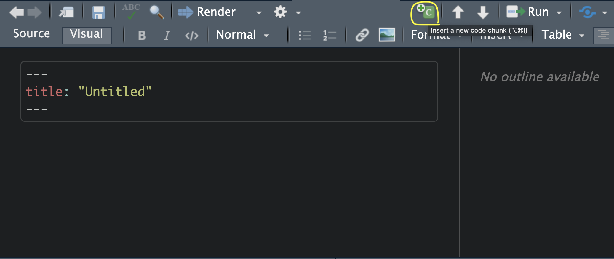
On the top right of the RStudio editor, you can see a green C button with a + sign. That button allows you to insert a code chunk in your document. See Figure 4.1.
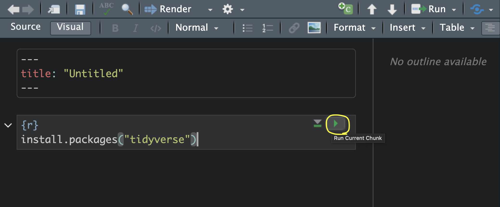
Then after you write your code and when you want to run the code in a chunk, you can click on the green Run button on the right side of the chunk. See Figure 4.2.
When you are working in a simple R script, you don’t need to worry about chunks. You can simply write your code in the script file and select the lines of code you want to run and click on the Run button.
Packages in R are like apps for your phone. Just like your phone comes with some basic apps, R comes with 14 base packages (as of May 11, 2024) including base, utils, and stats. But you can, and you will need to, install other packages to do different things just like you install apps on your phone.
You can install a package using the install.packages() function. This book uses the tidyverse package, which is a universe of packages that follow a common “tidy” data philosophy.
You can install the tidyverse package using the following command:
# uncomment the following line by removing "#" and run the code to install the tidyverse package

# install.packages("tidyverse")
You need to install the packages you need only once, and then you can use them whenever you want.
Just like apps on your phone, you need to load the packages you need every time you start a new R session. You can load the package using the library() function. For example, to load the tidyverse package, you can use the following command:
The [tidyverse](https://tidyverse.org/) package is a collection of packages including ggplot2, dplyr, tidyr, readr, purrr, tibble, stringr, forcats, rvest, lubridate, and a few other packages. We learn some of these packages in this book. Once you load the tidyverse package, you can use all the functions in these packages. In other words, you don’t need to load, for example, the ggplot2 package separately by running library(ggplot2).
You can assign values to variables in R using the <- operator. For example, you can assign the value 14 to a variable x using the following command:
x <- 14After assigning 14 to x, you can use x in your code. For example, you can print the value of x using the following command:
print(x)[1] 14See, x is now 14. You can also see the value of x by typing x in the console and pressing Enter. Try it.
x[1] 14You can also make additional data manipulations using x and assign it to another variable y using the following command:
y <- x + 3Let’s see the value of y:
y[1] 17R is an advanced calculator. You can do all kinds of calculations using R. For example, check out the following calculations:
# Square root of 16
sqrt(16)
[1] 4# 2 to the power of 8
2^8[1] 256# Logarithm of 100
log(100)[1] 4.60517# Exponential of previously assigned value y, i.e. 17, times x, i.e. 14.
exp(y) * x[1] 338169339You can also assign a character string to a variable. For example, you can assign the string “한국학 학자들 및 학생들도 R 좀 배웠으면 좋겠다.” to a variable z using the following command:
z <- "한국학 학자 및 학생들도 R 좀 배웠으면 좋겠다."You can print the value of z using the following command:
z[1] "한국학 학자 및 학생들도 R 좀 배웠으면 좋겠다."As a novice R user, more often than not, you will get error messages because you make mistakes in spelling. For example, we assigned the value 14 to a variable x. If you try to print the value of X instead of x, you will get an error message. Try it.
# Uncomment the following line by removing "#" and run the code to see the error message.

# X
You will get an error message saying that “Error: object ‘X’ not found”. This is because R is case-sensitive. X is not the same as x. Make sure to get the spelling right.
If you want to use more than two words for a variable name, you can use an underscore _ (my_variable) or a dot . (my.variable) to separate the words; or you can write the words together with each new word beginning with a capital letter (myVariable). You better be consistent with your naming convention, although technically you can name your variables however you want. For example, you can assign c("한국", "일본", "미국", "중국") to a variable my_variable using the following command:
my_variable <- c("한국", "일본", "미국", "중국")R has several data types including numeric, character, logical, date, list, dataframe and so on. Let’s see the data types of the variables we created above. We can use the class() function to see the data type of a variable. For example, you can see the data type of x, y, and z using the following commands:
The data type of x and y is numeric, and the data type of z is character.
If we write numbers in quotes, they become character strings. For example, you can assign the string “14” to a variable w using the following command:
w <- "14"You can see the data type of w using the following command:
class(w)[1] "character"The data type of w is character. You can also turn it into a numeric value using the as.numeric() function. For example, you can turn w into a numeric value using the following command:
w <- as.numeric(w)A vector is a collection of elements of the same data type. You can create a vector using the c() function. For example, you can create a vector v with the elements “서울”, “부산”, “대구”, “인천”, and “대전” using the following command:
v <- c("서울", "부산", "대구", "인천", "대전")You can print the vector v using the following command:
v[1] "서울" "부산" "대구" "인천" "대전"You can see the data type of v using the following command:
class(v)[1] "character"The data type of v is character. You can also create a numeric vector. For example, you can create a vector numbers with the elements 1, -2, 3.1, 49, and 0 using the following command:
numbers <- c(1, -2, 314, -49, 0)You can print the vector numbers using the following command:
numbers[1] 1 -2 314 -49 0You can see the data type of numbers using the following command:
class(numbers)[1] "numeric"The data type of numbers is numeric.
A dataframe is a collection of vectors of the same length. You can create a dataframe using the data.frame() function. For example, you can create a dataframe df with three columns city_name_en, city_name_kr, and population using the following command:
# Relying on this link for the population data (in millions):
# https://kosis.kr/statHtml/statHtml.do?orgId=101&tblId=DT_1B040A3

df <- data.frame(city_name_en = c("Busan", "Daegu", "Incheon", "Seoul", "Daejeon"),
                 city_name_kr = c("부산", "대구", "인천", "서울", "대전"),
                 population = c(3.3, 2.4, 3, 9.4, 1.4))
You can print the dataframe df using the following command:
df city_name_en city_name_kr population
1 Busan 부산 3.3
2 Daegu 대구 2.4
3 Incheon 인천 3.0
4 Seoul 서울 9.4
5 Daejeon 대전 1.4You can see the data type of df using the following command:
class(df)[1] "data.frame"The data type of df is dataframe. We can reach the columns of the dataframe using the $ sign. For example, you can see the column city_name_en using the following command:
df$city_name_en[1] "Busan" "Daegu" "Incheon" "Seoul" "Daejeon"You can use the head() function to see the first few rows of a dataframe. For example, you can see the first few rows of the dataframe df using the following command:
head(df) city_name_en city_name_kr population
1 Busan 부산 3.3
2 Daegu 대구 2.4
3 Incheon 인천 3.0
4 Seoul 서울 9.4
5 Daejeon 대전 1.4By default, the head() function shows the first 6 rows of the dataframe. You can also specify the number of rows you want to see. For example, you can see the first 3 rows of the dataframe df using the following command:
head(df, 3) city_name_en city_name_kr population
1 Busan 부산 3.3
2 Daegu 대구 2.4
3 Incheon 인천 3.0You can use the tail() function to see the last few rows of a dataframe. For example, you can see the last few rows of the dataframe df using the following command:
tail(df) city_name_en city_name_kr population
1 Busan 부산 3.3
2 Daegu 대구 2.4
3 Incheon 인천 3.0
4 Seoul 서울 9.4
5 Daejeon 대전 1.4In this example, both the head() and tail() functions show the entire dataframe because the dataframe df has only 5 rows. But, in longer dataframes, you can see the first or last few rows using these functions.
In a similar vein, glimpse() function from the dplyr package is a function to see the structure of a dataframe. For example, you can see the structure of the dataframe df using the following command:
glimpse(df)Rows: 5
Columns: 3
$ city_name_en <chr> "Busan", "Daegu", "Incheon", "Seoul", "Daejeon"
$ city_name_kr <chr> "부산", "대구", "인천", "서울", "대전"
$ population <dbl> 3.3, 2.4, 3.0, 9.4, 1.4The nrow() function gives the number of rows in a dataframe. For example, you can see the number of rows in the dataframe df using the following command:
nrow(df)[1] 5Likewise, the ncol() function gives the number of columns in a dataframe. For example, you can see the number of columns in the dataframe df using the following command:
ncol(df)[1] 3The dim() function gives the dimensions of a dataframe. For example, you can see the dimensions of the dataframe df using the following command:
dim(df)[1] 5 3The summary() function gives a summary of a dataframe. For example, you can see the summary of the dataframe df using the following command:
summary(df) city_name_en city_name_kr population
Length:5 Length:5 Min. :1.4
Class :character Class :character 1st Qu.:2.4
Mode :character Mode :character Median :3.0
Mean :3.9
3rd Qu.:3.3
Max. :9.4 You can select rows and columns of a dataframe using the [] operator. The first argument of the [] operator is the row index, and the second argument is the column index. df[row, column] selects the row with the index row and the column with the index column.
For example, you can select the first row and the second column of the dataframe df using the following command:
df[1, 2][1] "부산"You can select the first row of the dataframe df using the following command:
df[1, ] city_name_en city_name_kr population
1 Busan 부산 3.3You can select the second column of the dataframe df using the following command:
df[, 2][1] "부산" "대구" "인천" "서울" "대전"The pipe operators |> and %>% are powerful tools in R.1 The pipe allows you to write code in a more readable way. You can use the pipe operator to pass the output of one function to the input of another function. For example, you can use the pipe operator to pass the dataframe df to the head() function. You can see the first few rows of the dataframe df using the following command:
df |> head() city_name_en city_name_kr population
1 Busan 부산 3.3
2 Daegu 대구 2.4
3 Incheon 인천 3.0
4 Seoul 서울 9.4
5 Daejeon 대전 1.4We can arrange the dataframe df using the arrange() function from the dplyr package. For example, you can arrange the dataframe df by the population column using the following command with a pipe:
df |> arrange(population) city_name_en city_name_kr population
1 Daejeon 대전 1.4
2 Daegu 대구 2.4
3 Incheon 인천 3.0
4 Busan 부산 3.3
5 Seoul 서울 9.4arrange() function arranges the dataframe by the selected numeric column in ascending order by default. If it is a character column, it arranges the dataframe in alphabetical order. You can arrange the dataframe in descending order by using the desc() function. For example, you can arrange the dataframe df by the population column in descending order using the following command:
  city_name_en city_name_kr population
1        Seoul         서울        9.4
2        Busan         부산        3.3
3      Incheon         인천        3.0
4        Daegu         대구        2.4
5      Daejeon         대전        1.4
We can also assign df to the rearranged dataframe. For example, you can assign the arranged dataframe to df using the following command:
Now, df is arranged by the population column in descending order. Let’s check out:
df city_name_en city_name_kr population
1 Seoul 서울 9.4
2 Busan 부산 3.3
3 Incheon 인천 3.0
4 Daegu 대구 2.4
5 Daejeon 대전 1.4Good. We learned the basics of R. In the next chapter, we learn about data wrangling using mainly the dplyr package.